PostGIS is an extension to Postgres to manage geospatial data. PostGIS supports rasters data (images) and vector data (lines, polygons), operations on rasters and vectors, geospatial indexes, different projections, and more.

We used PostGIS at Airspace Intelligence as a base for a service that would serve generic airspace-related information, both in vector format (e.g. closed airspace) and raster format (e.g. weather maps).

It turned out a non-trivial task to build such a generic and performant service. Here I want to share some lessons that we learned along.

Performance on vector data

The title of this blog post says “raster maps” and the rest of the post circles around that topic. It is because the single lesson learned related to handling vector data is that PostGIS is extremely performant when it comes to processing and serving vector data. It’s enough that you put all your vector data into the database and serve it directly from the database without any additional tricks.

GDAL, out-db, and Google Cloud SQL compatibility

PostGIS uses GDAL (Geospatial Data Abstraction Library), which is a battle-proven library and a set of great tools to transform data between different projections and formats, perform operations on geographical rasters, and more.

PostGIS with raster drivers is an extremely versatile and flexible tool for prototyping. You can very easily load the datasets to the database, intersect coordinates, and output the datasets to different formats with a bunch of SQL lines.

GDAL, and therefore PostGIS, offers “out-db” drivers to store the raster images outside of the database. Out-db allows storing the heavy raster image in Google Cloud Store, AWS S3 or a local file. The database will store only a reference (a URI) to the remote asset together with other metadata (e.g. bounding box), dramatically reducing table size (instead of storing 1MB image it stores only 1KB of metadata). All the operations on rasters are transparent, GDAL will take care of fetching and processing the remote assets.

While bootstrapping Google Cloud SQL and PostGIS we bitterly realized that Google Cloud SQL does not support PostGIS Drivers (see this ticket and the drivers here and here). This means that if you want to use built-in GDAL goodies for rasters and out-db in Google Cloud Platform, you need to sacrifice all the automation that Cloud SQL offers and manage your own PostGIS instance.

Further, when using out-db we encountered a blocking bug. While most of the time out-db and Google Cloud Store (GCS) worked flawlessly, sometimes it just didn’t. The database querying the objects in GCS randomly failed (around 1% of the requests, IIRC). We were not able to track down the root cause and were forced to abandon out-db in favor of our own image management. We ruled out network issues and GCS request rate limit issues, we were looking inside the GDAL source code just to stop at the line saying that the file did not exist.

We worked the issue around by leaving out-db and managing the files on our own. Basically, we implemented a mechanism akin to out-db but in the application. We left exactly the same database and GCS layout, but instead of fetching the data through out-db, we fetched the data directly in the application. Handling the raster files in the application, and not in the database, enabled us to optimize further by caching the frequently accessed data in Redis, and also caching the whole queries.

Worth noting that while we abandoned the original integration of GDAL and GCS, we still preserved the original format of all the data in the database. This was useful because we still could use raster2pgsql and all the PostGIS queries to prototype and troubleshoot.

Another lesson learned was that GDAL toolchain and raster2pgsql tool in particular are great. You can easily load the rasters to the database using a variety of input formats and apply predefined transformations gdal_warp and gdal_translate or you can apply arbitrary custom transformations defined with Python using gdal_calc. Those tools are particularly handy when working with GRIB2 or NetCDF input formats.

Raster processing

Other lessons learned were related to the performance of processing of the rasters. In particular, we were interested in coloring layers and merging different colored layers onto a single raster.

As it turned out, PostGIS raster processing can be prohibitively slow. Any non-trivial operations on rasters, or operations on multiple rasters, that eventually use ST_MapAlgebra, are just slow for an online application with a snappy interface. We eventually had to implement our own raster operations on the application side in numpy, which gave us speed and flexibility.

The flexibility of processing rasters in numpy was useful also because we encountered problems with the ST_Clip operation. ST_Clip, possibly due to a bug, or us not using it properly, produced an artifact when used together with ST_Resample. When we were clipping a large raster to a small tile, ST_Clip left a strip of transparent pixels at the edge, that we were not able to get rid of. I suppose that it was a rounding error at the edge of the tile since to resample you need to “look around” and there might not be any “around” at the edge of the clipped image. Eventually, since we moved raster processing to numpy, we worked the problem around.

Example of the bug which resulted in an empty strip.

Processing the rasters on the application side opened a path to optimizations. One optimization was to shrink the raster images stored on GCS so those images are faster to download and, in the long run, cheaper to store. The images contained values of weather models (like reflectivity, which is a proxy of precipitation). While the original value was float, for visualization purposes we did not need such a large dynamic of the signal. Scaling the original values to fit 8 bits per pixel together with LZW lossless compression reduced the storage size significantly. This optimization led to a quirky bug. By default, PostGIS treat 255 as a “no value” value. When the function compressing the values capped the maximum compressed pixel value at 255, the result was that those 255s showed up as holes in the images. Capping the values at 254 solved the issue.

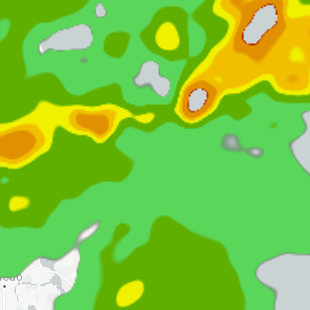
The picture shows the holes in the large values at the top-right, where the large values are colored red.

Query optimizations

Another hard-won lesson was that the careful using of CTEs in PostGIS can boost, or ditch, performance. Especially, for some queries, PostGIS did not use the geospatial index optimally. Manually marking some CTEs as “materialized” or “not materialized” changed the query from barely usable to blazing fast.

Also worth noting, the Postgres query planner does not optimize custom functions, so for performance, we had to inline in the queries (this was for the raster processing functions that we eventually abandoned).

Python interoperability

When we were experimenting with doing the raster processing entirely in the database, we had to expose the rasters from PostGIS to Python. One could expose the queried values with ST_DumpValues, but it turned out to be prohibitively slow. Using the raw WKB format (”Well Known Binary”, what a great acronym) is far faster but requires parsing WKB in Python. Fortunately the format is easy to parse. If you try to parse WKB yourself, you will probably stumble upon this example. Beware, it’s buggy, it does not recognize the “nodata” value, therefore, all the values are shifted by one pixel.

Conclusions

PostGIS is a great tool, although it can be slow when you want to have any non-trivial raster processing. To process rasters you are better off processing the images on the application side. Also, the integration of PostGIS and Google Cloud Platform can cause problems.

Acknowledgments

Thanks Lucas Kukielka for proofreading and comments!

(HN)